Getting Started With qtcm

Your First Model Run

Figure 3.1 shows an example of a script to make a 30 day seasonal, aquaplanet model run, with run name ``test'', starting from November 1, Year 1.

$\parbox{70ex}{\footnotesize{% \textcolor{blue}{\texttt{% from qtcm ... ...led\_form'] = 'parts' \\ model = Qtcm(**inputs) \\ model.run\_session()}} }}$

$\parbox{70ex}{\footnotesize{Figure~\re... ...g:my.first.run}: An example of a simple \textcolor{blue}{\texttt{qtcm}} run.}}$

The class describing the QTCM1 model is Qtcm. An instance of Qtcm, in this example model, is created the same way you create an instance of any class. When instantiating an instance of Qtcm, keyword parameters can be used to override any default settings. In the example above, the dictionary inputs specifying all keyword parameters is passed in on the instantiation of model.

The keyword parameter settings in Figure 3.1 have the following meanings:

• runname: This string (``test'') is used in the output filename. QTCM1 writes mean and instantaneous output files to the directory given in model.outdir.value, with filenames qm_runname.nc for mean output and qi_runname.nc for instantaneous output.

• landon: When set to ``0'', the land is turned off and the run is an aquaplanet run. When set to ``1'', the land model is turned on.

• year0: The year the run starts on.

• month0: The month the run starts on (11 = November).

• day0: The day of the month the run starts on.

• lastday: The model runs from day 1 to lastday.

• mrestart: When set to ``0'', the run starts from default initial conditions (see Section 4.7.2 for a table of those values). When set to ``1'', the run starts from a restart file.

• compiled_form: This keyword sets what form the compiled QTCM1 model has, and its value is saved to the instance's compiled_form attribute. It is a string and can be set either to ``parts'' or ``full''. Most of the time, you will want to set it to 'parts'. This keyword is the only one that must be specified on instantiation; the model instance will at least instantiate using only the default settings for all the other keyword parameters (given in Appendix A). See Section 4.4 for details about what the compiled_form attribute controls.

By default, the SSTmode attribute, which controls whether the model will use climatological sea-surface temperatures (SST) or real SSTs, is set to the value ``seasonal'', thus giving a run with seasonal forcing at the lower-boundary over the ocean.

This example assumes that the boundary condition files, sea surface temperature files, and the model output directories are as specified in submodule defaults. Those values are described in Section A.1.

Managing Directories

Most of the time, your boundary condition files and output files will not be in the locations specified in Section A.1, or in the directory your Python script resides. The easiest way to tell your Qtcm instance where your input/output files are is to pass them in as keyword parameters on instantiation.

$\parbox{70ex}{\footnotesize{% \textcolor{blue}{\texttt{% from qtcm ... ...led\_form'] = 'parts' \\ model = Qtcm(**inputs) \\ model.run\_session()}} }}$

$\parbox{70ex}{\footnotesize{Figure~\re... ...ttt{qtcm}} run showing detailed description of input and output directories.}}$

Figure 3.2 shows an example run where those directories are explicitly specified; in all other aspects, the run is identical to the one in Figure 3.1. In Figure 3.2, output from the model is directed to the directory described by string variable dirbasepath. dirbasepath is created by joining the current working directory with the run name given in string variable rundirname.^3.1Setting keyword parameter outdir to dirbasepath sends output to dirbasepath. Keywords bnddir and SSTdir specify the directories where non-SST and SST boundary condition files, respectively, are found.

Interestingly, the default version of QTCM1 does not send all output from the model to outdir. The restart file qtcm_yyyymmdd.restart (where yyyymmdd is the year, month, and day of the model date when the restart file was written) is written into the current working directory, not the output directory. Thus, if you do multiple runs, you'll have to manually deal with the restart files that will proliferate.

Neither the QTCM1 model nor the Qtcm object create the directories specified in bnddir, SSTdir, and outdir. Failure to do so will create an error. I use Python's file management tools to make sure the output directory is created, and any old output files are deleted. Here's an example that does that, using the dirbasepath and rundirnamevariables from Figure 3.2:

if not os.path.exists(dirbasepath): os.makedirs(dirbasepath)
qi_file = os.path.join( dirbasepath, 'qi_'+rundirname+'.nc' )
qm_file = os.path.join( dirbasepath, 'qm_'+rundirname+'.nc' )
if os.path.exists(qi_file): os.remove(qi_file)
if os.path.exists(qm_file): os.remove(qm_file)

Model Field Variables

The term ``field'' variable refers to QTCM1 model variables that are accessible at both the compiled Fortran QTCM1 model-level as well as the Python Qtcm instance-level. Field variables are all instances of the Field class, and are stored as attributes of the Qtcm instance.^3.2

Field class instances have the following attributes:

• id: A string naming the field (e.g., ``Qc'', ``mrestart''). This string should contain no whitespace.
• value: The value of the field. Can be of any type, though typically is either a string or numeric scalar or a numeric array.
• units: A string giving the units of the field.
• long_name: A string giving a description of the field.

Field instances also have methods to return the rank and typecode of value.

Remember, if you want to access the value of a Field object, make sure you access that object's value attribute. Thus, for example, to assign a variable foo to the lastday value for a given Qtcm instance model, type the following:

foo = model.lastday.value

For scalars, this assignment sets foo by value (i.e., a copy of the value of attribute model.lastday is set to foo). In general, however, Python assigns variables by reference. Use the copy module if you truly want a copy of a field variable's value (such as an array), rather than an alias. For more details about field variables, see Section 4.7.

Run Sessions

What is a Run Session?

A run session is a unit of simulation where the model is run from day 1 of simulation to the day specified by the lastdayattribute of a Qtcm instance. A run session is a ``complete'' model run, at the beginning of which all compiled QTCM1 model variables are set to the values given at the Python-level, and at the end of which restart files are written, the values at the Python-level are overwritten by the values in the Fortran model, and a Python-accessible snapshot is taken of the model variables that were written to the restart file.

Changing Variables

Between run sessions, changing any field variable is as easy as a Python assignment. For instance, to change the atmosphere mixed layer depth to 100 m, just type:

model.ziml.value = 100.0

When changing arrays, be careful to try to match the shape of the array.^3.3You can use the NumPy shape function on a NumPy array to check its shape.

Continuing a Model Run

Figure 3.3 shows an example of two run sessions, where the second run session is a continuation of the first.

$\parbox{70ex}{\footnotesize{% \textcolor{blue}{\texttt{% inputs['ye... ... model.init\_with\_instance\_state = True \\ model.run\_session(cont=30)}} }}$

$\parbox{70ex}{\footnotesize{Figure~\re... ...name and all input and output directory names were added to the dictionary.}}$

The first run session runs from day 1 to day 10. The second run session runs the model for another 30 days. Setting the init_with_instance_state of model to True tells the model to use the the values of the instance attributes (for prognostic variables, right-hand sides, and start date) are currently stored modelas the initial values for the run_session.^3.4The contkeyword in the second run_session call specifies a continuation run, and the value gives the number of additional days to run the model.

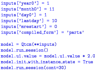
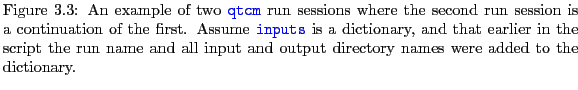
The set of runs described above would produce the exact same results as if you had gone into the Fortran model after 10 days, doubled the first baroclinic mode zonal velocity, and continued the run for another 30 days. With the Python example above, however, you didn't need to know you were going to do that ahead of starting the model run (which is what a compiled model requires you to do). Section 4.5 describes continuation runs in detail.

Passing Restart Snapshots Between Run Sessions

The pure-Fortran QTCM1 uses a restart file to enable continuation runs. A Qtcm instance can also make use of that option, through setting the mrestart attribute value (see Section 4.5 and Neelin et al. [4] for details). It's easier, however, instead of using a restart file, to pass along a ``snapshot'' dictionary.

The Qtcm instance method make_snapshot copies the variables that would be written out to a restart file into a dictionary that is saves as the instance attribute snapshot. This snapshot can be saved separately, for later recall. Note that snapshots are automatically made at the end of a run session.

The following example shows a model run_session call, following which the snapshot is saved to the variable snapshot:^3.5

model.run_session()
mysnapshot = model.snapshot

After taking the snapshot, you might continue the run a while, and then decide to return to the snapshot you saved. To do so, use the sync_set_py_values_to_snapshotmethod to reset the model instance values to mysnapshot before your next run session:

model.sync_set_py_values_to_snapshot(snapshot=mysnapshot)
model.init_with_instance_state = True
model.run_session()

See Section 4.5.5 for details regarding the use of snapshots, as well as for a list of what variables are saved in a snapshot.

Creating Multiple Models

Model Instances

Creating a new QTCM1 model is as simple as creating another Qtcm instance. For instance, to instantiate two QTCM1 models, model1 and model2, type the following:

from qtcm import Qtcm
model1 = Qtcm(compiled_form='parts')
model2 = Qtcm(compiled_form='parts')

model1 and model2 do not share any variables in common, including the extension modules holding the Fortran code. In creating the instances, a copy of the extension modules are saved in temporary directories.

Passing Snapshots To Other Models

The snapshots described in Section 3.4.4 can also be passed around to other model instances, enabling you to easily branch a model run:

model.run_session()
mysnapshot = model.snapshot
model1.sync_set_py_values_to_snapshot(snapshot=mysnapshot)
model2.sync_set_py_values_to_snapshot(snapshot=mysnapshot)
model1.run_session()
model2.run_session()

The state of model after its run session is used to start model1 and model2. This is an easy way to save time in spinning-up multiple models.

Run Lists

This feature of Qtcm objects is what really gives Qtcm model instances their flexibility. A run list is a list of strings and dictionaries that specify what routines to run in order to execute a particular part of the model. Each element of the run list specifies the method or subroutine to execute, and the order of the elements specifies their execution order.

For instance, the standard run list for initializing the the atmospheric portion of the model is named ``qtcminit'', and equals the following list:

['__qtcm.wrapcall.wparinit',
'__qtcm.wrapcall.wbndinit',
'varinit',
{'__qtcm.wrapcall.wtimemanager': [1]},
'atm_physics1']

This list is stored as an entry in the runlists dictionary (with key 'qtcminit'). runlists is an attribute of a Qtcm instance. Table 4.3 lists all standard run lists.

When the run list element in the list is a string, the string gives the name of the routine to execute. The routine has no parameter list. The routine can be a compiled QTCM1 model subroutine for which an interface has been written (e.g., __qtcm.wrapcall.wparinit), a method of the of the Python model instance (e.g., varinit), or another run list (e.g., atm_physics1).

When the run list element is a 1-element dictionary, the key of the dictionary element is the name of the routine, and the value of the dictionary element is a list specifying input parameters to be passed to the routine on call. Thus, the element:

{'__qtcm.wrapcall.wtimemanager': [1]}

calls the __qtcm.wrapcall.wtimemanager routine, passing in one input parameter, which in this case is the value 1.

If you want to change the order of the run list, just change the order of the list. To add or remove routines to be executed, just add and remove their names from the run list. Python provides a number of methods to manipulate lists (e.g., append). Since lists are dynamic data types in Python, you do not have to do any recompiling to implement the change.

The compiled_form attribute must be set to 'parts'in the Qtcm instance in order to take advantage of the run lists feature of the class. Run lists are not available for compiled_form='full', because subroutine calls are hardwired in the compiled QTCM1 model Fortran code in that case.

Model Output

NetCDF Output

Model output is written to netCDF files in the directory specified by the Qtcm instance attribute outdir. Mean values are written to an output file beginning with qm_, and instantaneous values are written to an output file beginning with qi_.

The frequency of mean output is controlled by ntout, and the frequency of instantaneous output is controlled by ntouti. ntout.value gives the number of days over which to average (and if equals -30, monthly means are calculated). ntouti.value gives the frequency in days that instantaneous values are output (monthly if it equals -30). (See Section 4.7.2 for a description of other output-control variables, and see the QTCM1 manual [4] for a detailed description of how these variables control output.)

Figure 3.4 gives an example of a block of code to read netCDF output, where datafn is the netCDF filename, and id is the string name of the field variable (e.g., 'u1', 'T1', etc.). (Note that the netCDF identifier for field variables is the same as the name in Qtcm, except for the variables given in Table 3.1.)

In the code in Figure 3.4, the array value is read into data, and the longitude values, latitude values, and time values are read into variables lon, lat, and time, respectively. As netCDF files also hold metadata, a description and the units of the variable given by id, and each dimension, are read into variables ending in _name and _units, respectively.

$\parbox{70ex}{\footnotesize{% \textcolor{blue}{\texttt{% import num... ... \\ time\_units = fileobj.variables['time'].units \\ \\ fileobj.close()}} }}$

$\parbox{70ex}{\footnotesize{Figure~\re... ...d}: Example of Python code to read netCDF output. See text for description.}}$

Table: NetCDF output names for Qtcm field variables that are different from the Qtcm and compiled QTCM1 model variable names. The netCDF names are case-sensitive.

Qtcm Attribute Name	NetCDF Output Name
'Qc'	'Prec'
'FLWut'	'OLR'
'STYPE'	'stype'

NB: All netCDF array output is dimensioned (time, latitude, longitude) when read into Python using the Scientific package. This differs from the way Qtcm saves field variables, which follows Fortran convention (longitude, latitude). Please be careful when relating the two types of arrays. Section 4.7.4 for a discussion of why there is this discrepancy.

Visualization

The plotm method of Qtcm instances creates line plots or contour plots, as appropriate, of model output of average fields of run session(s) associated with the instance. Some examples, assuming model is an instance of Qtcmand has already executed a run session:

• model.plotm('Qc', lat=1.875): A time vs. longitude contour plot is made for the full range of time and longitude, at the latitude 1.875 deg N, for mean precipitation.

• model.plotm('Qc', time=10): A latitude vs. longitude contour plot of precipitation is made for the full spatial domain at day 10 of the model run.

• model.plotm('Evap', lat=1.875, lon=[100,200]): A contour plot of time vs. longitude of evaporation is made for the longitude points between 100 and 200 degrees E, at the latitude 1.875 deg N.

• model.plotm('cl1', lat=1.875, lon=[100,200], time=20): A deep cloud amount vs. longitude line plot is made for the longitude points between 100 and 200 degrees east, at the latitude 1.875 deg N, at day 20 of the model run.

In these examples, the number of days over which the mean is taken equals model.ntout.value. Also, the plotm method automatically takes into account the Qtcm/netCDF variable differences described in Table 3.1.

Documentation

Section 1.4 gives the online locations of the transparent copies of this manual. Model formulation is fully described in Neelin & Zeng [3] and model results are described in Zeng et al. [5] ([3] is based upon v2.0 of QTCM1 and [5] is based on QTCM1 v2.1). Additional documentation you'll find useful include:

• The qtcm Package API Documentation

• The Pure-Fortran QTCM1 Manual [4]